NeuroMatrix

Why this matters

Most neural network hardware today is digital, dense, and synchronous: matrix multiplies on a GPU, every neuron updating every clock cycle whether it has anything to say or not. That works, and it’s why GPT-5 exists. But it’s also why training a frontier model costs tens of millions of dollars in electricity, and why doing useful inference on a small device is still hard.

Biological brains aren’t dense or synchronous. A neuron fires when it has something to communicate and stays quiet otherwise, and the signal it sends — a spike — is a single event in time, not a continuous activation. The network is event-driven: power is spent only when computation actually happens. Estimates vary, but the brain runs at something like 20 watts, which is less than the laptop I’m typing this on.

Spiking neural networks (SNNs) try to capture this. Analog SNNs go further: instead of digitally simulating spiking dynamics, the neurons are actual circuits — capacitors charging, currents leaking, transistors switching — that are the dynamics. The membrane voltage of a silicon neuron isn’t a float32; it’s a real voltage on a real capacitor. The leak isn’t modeled; it’s a real subthreshold current through a real MOSFET.

NeuroMatrix is one bet on what an analog SNN should look like at scale, how to validate it before paying for silicon, and what to build on top of it once you have it.

What we built

The project has three parts that you can read as separable contributions or as one system:

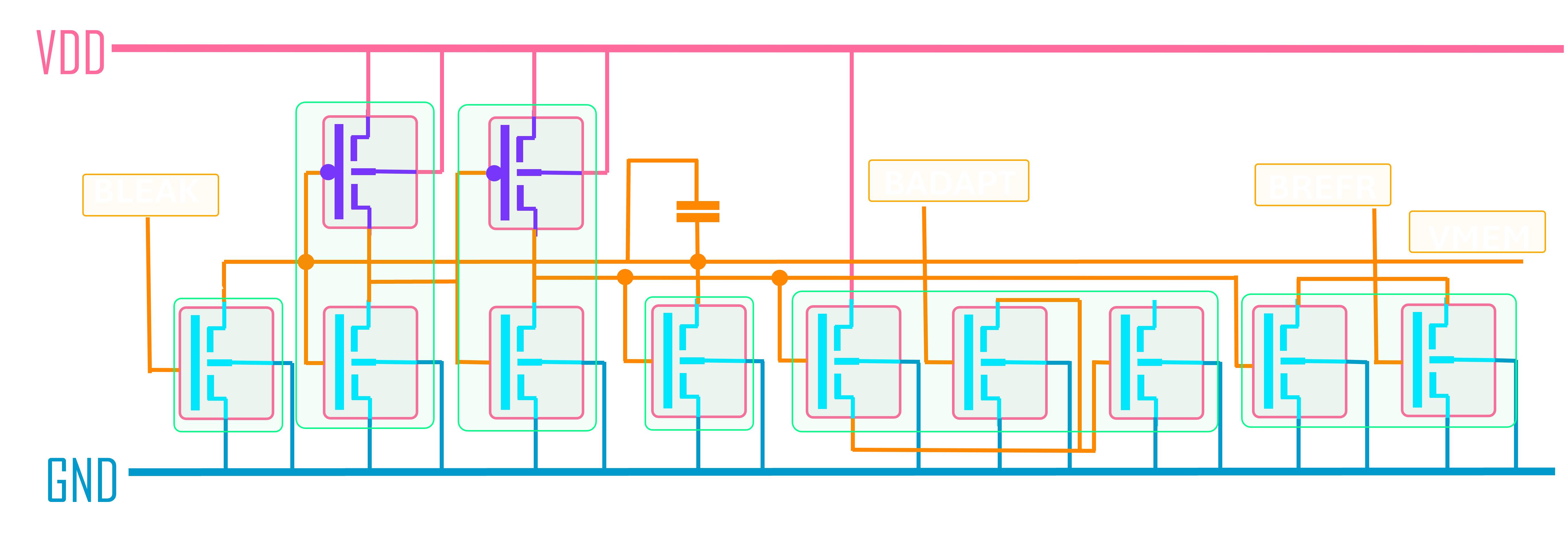
1. A neuron circuit — an Axon-Hillock leaky integrate-and-fire (LIF) topology with 11 transistors plus a feedback capacitor, designed for IHP’s SG13G2 BiCMOS process and validated in foundry PSP 103.6 models.
2. A simulation framework with three-level verification — Python prototyping, C++ at network scale, Rust hosting the Circuit IR and Fabrica bindings; the same network description exercised at scales from 300 to 25,100 neurons, with EKV-2.6 transistor-level checks and PSP103 foundry SPICE for circuit sign-off.
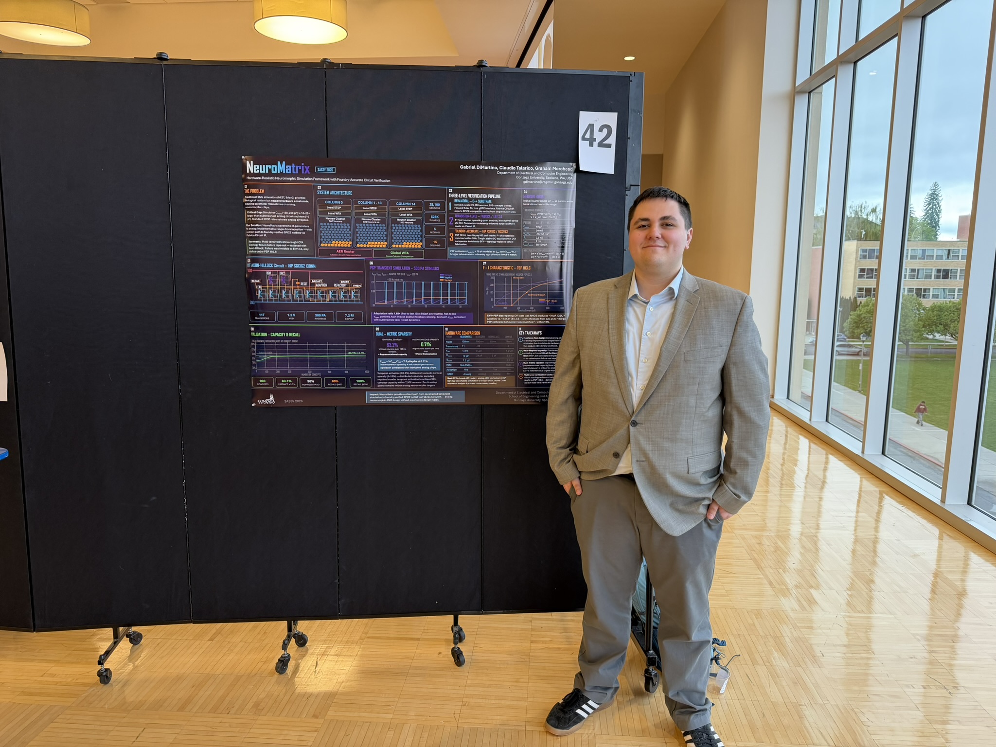
3. An application — sparse associative memory. The network stores 993 distinct concepts and recalls them from partial cues, validating both the circuit and the framework against a meaningful cognitive task. This is the ASSOCIATIVE region of a larger cognitive architecture (NeuroCog) that includes sequential, logic, causal, and planning regions, with parallel cognitive modules — Linguistic, Generative, Episodic — being built on the same substrate.

The paper covers the circuit, the framework, and the associative memory result. This writeup walks through those, plus the encoding pipeline that gets text into spike patterns and the cognitive stack being built on top.

The circuit

The neuron is an Axon-Hillock LIF topology. The name comes from the part of a biological neuron where action potentials are initiated — the integrating segment where graded membrane voltage gets converted into discrete spikes — and the circuit is a faithful analog of that mechanism condensed to silicon.

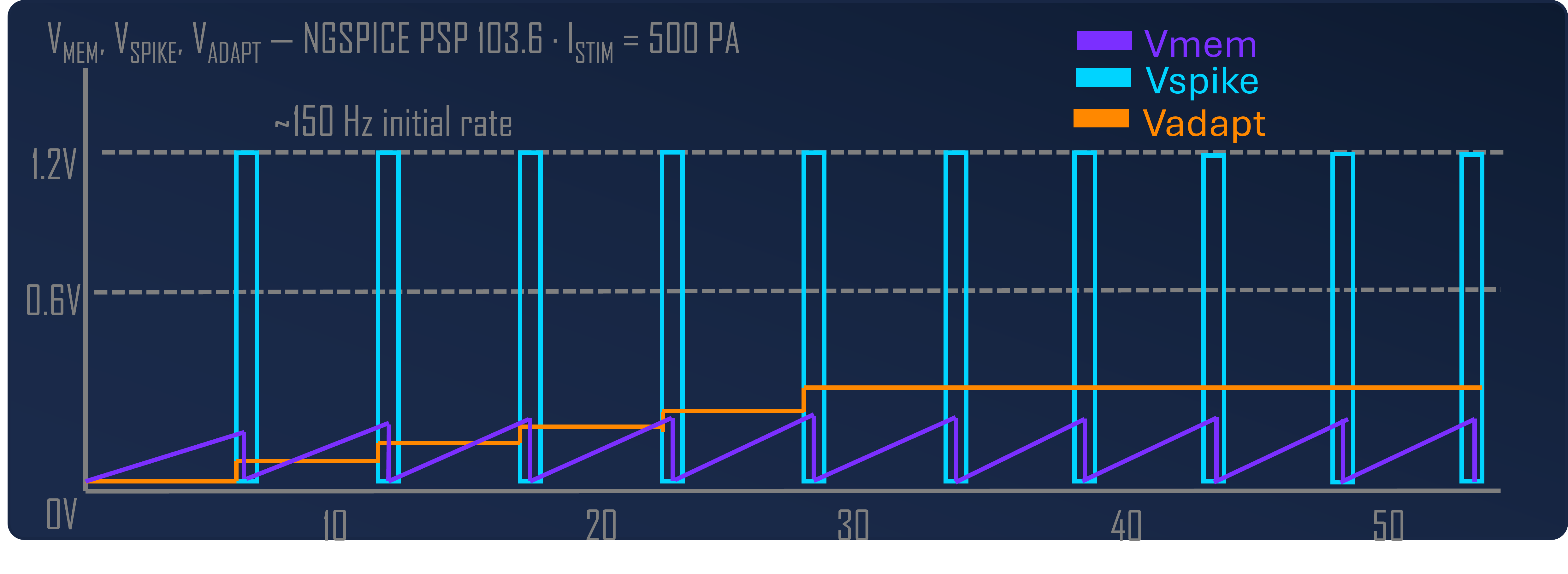
The eleven transistors break down into five functional groups. A subthreshold NMOS leak (W = 0.5 µm, L = 2 µm) sits at the membrane node and pulls charge off Cmem at a rate set by an externally programmable bias Vbleak; this gives the leaky integrator its time constant (τm = 20 ms, matching biological timescales). A CMOS inverter pair (INV1 + INV2, four transistors) acts as a non-inverting high-gain amplifier on the membrane voltage — when Vmem crosses INV1’s trip point (≈ 0.6 V), the inverter chain snaps and produces a clean digital spike. A reset switch (W = 2 µm) discharges Cmem after each spike. A 2-transistor refractory hold circuit pulls the membrane below threshold for ~2 ms after a spike, preventing immediate re-firing. A 3-transistor adaptation accumulator sources a current proportional to recent spike activity, giving the neuron frequency adaptation — at sustained 500 pA stimulus, the firing rate falls 1.68× from first to last interval over 500 ms.

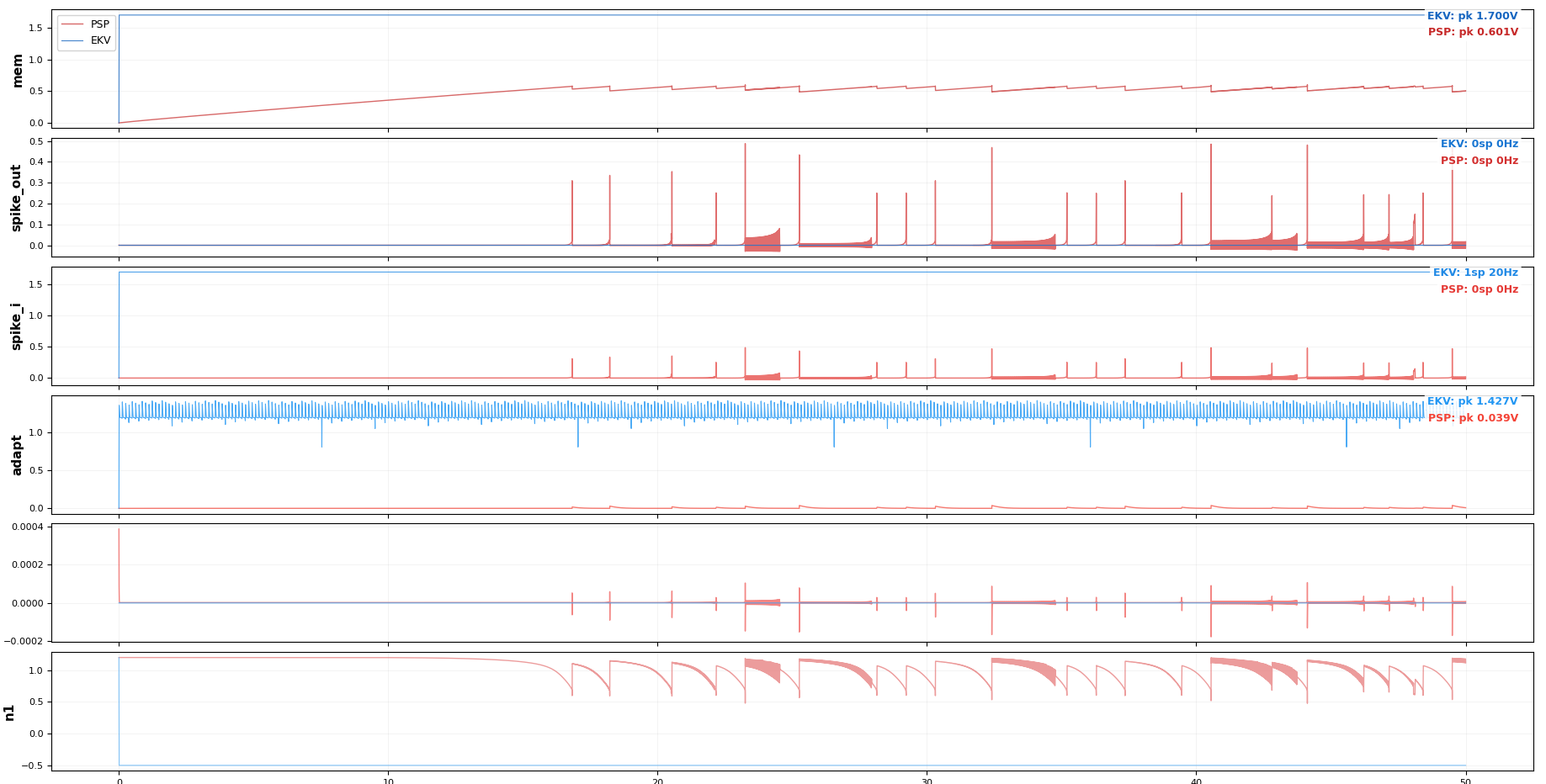
The eleventh element isn’t a transistor: it’s Cfb, a 1 pF feedback capacitor between INV2’s output and the membrane node. This is the part that makes the topology Axon-Hillock specifically. When the inverter pair triggers, Cfb injects a ~109 mV kick (VDD · Cfb / (Cmem + Cfb)) back into the membrane through capacitive coupling, latching the spike rail-to-rail rather than letting the membrane drift back through the trip point. It’s positive feedback in the cleanest possible form — no amplifier, no comparator hysteresis, just a capacitor — and it produces sharper, more energy-efficient spikes than alternatives like Indiveri’s OTA-based comparator topology (which an earlier version of the design used; PSP 103.6 validation later revealed a stable DC equilibrium in the OTA design invisible to EKV 2.6, and we revised to Axon-Hillock).

Why subthreshold operation matters: in subthreshold (Vgs < Vth), MOSFET drain currents are exponential in gate voltage rather than quadratic, the way they are in saturation. Drain currents in subthreshold land in the picoamp-to-nanoamp range. This is also exactly the range where biological neurons operate; the energetics of charging a 10 pF capacitor through a sub-nanoamp current naturally yield the millisecond-scale time constants you want for a brain-like network. Suprathreshold designs would be faster but would burn orders of magnitude more power and would lose the analog-to-biology mapping that makes the design choices defensible. Energy per spike comes out at ½·Cmem·VDD² = 7.2 pJ, with the dynamics dominated by capacitor charge/discharge rather than static current.

The choice of IHP SG13G2 as a process deserves a note. It’s a 130nm BiCMOS process — old, but in this context that’s a feature, not a bug. Analog circuits don’t get easier in smaller nodes: matching gets worse, leakage gets worse, supply voltages shrink until you can’t fit a useful signal swing. 130nm is a sweet spot for analog and especially for low-power neuromorphic work. IHP is also open about their PDK in a way most foundries aren’t, which matters if you want to share your design and verify other people’s results against the same models.

Three-level verification. The circuit isn’t validated by a single SPICE run. It’s validated three times, at progressively higher fidelity, by Fabrica’s verification pipeline:

1. Behavioral simulation in C++ at network scale (25,100 neurons, 993 concepts) — fast, lets us iterate on architecture and learning rules.
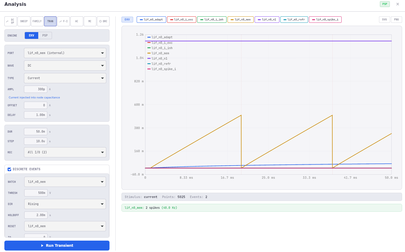
2. Transistor-level analysis via EKV 2.6 compact models in Fabrica-Viz — interactive operating-point exploration on a single neuron or small group, useful for tuning bias voltages and catching obvious topology errors.
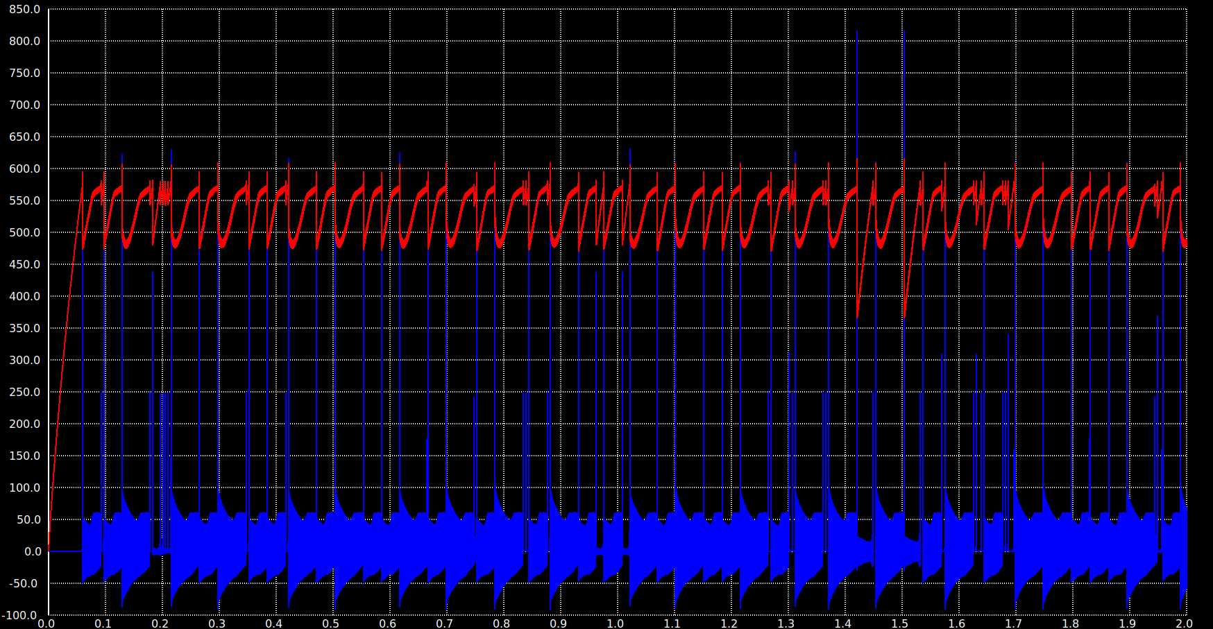
3. Foundry-accurate SPICE via IHP PSP103 models in ngspice — the actual sign-off check, run on the same Circuit IR netlist that the C++ behavioral layer was generated from.

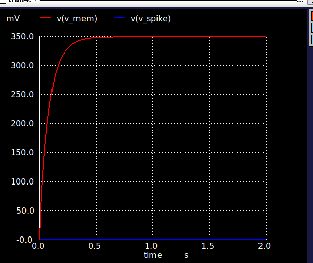
The value of this cascade was demonstrated by the OTA-to-Axon-Hillock revision mentioned above: EKV 2.6 was happy with the OTA topology, but PSP 103.6 — accounting for GIDL, junction leakage, and other effects the simpler model misses — revealed a stable DC equilibrium that would have killed the design in silicon. Multi-level verification caught it before fabrication. Under PSP 103.6, the leak MOSFET produces ~70 pA at Vgs = 0 V (versus < 1 pA in EKV 2.6), which shifts the effective rheobase from picoamps to ~300 pA. Fabrica’s PSP-calibrated behavioral mode now uses the extracted leak current to match the circuit’s F-I characteristic within 10%, bridging behavioral simulation to foundry sign-off.

The simulation framework

Building one neuron is straightforward. Building a network of 25,000 of them — in a way you can iterate on without burning silicon and without losing the connection to what the silicon will actually do — is the hard part. This is where the bulk of the engineering went.

The framework has three execution backends that share a single network description:

• Python — for rapid prototyping. Slow but readable; you can rewrite a learning rule in five minutes, sketch a new region’s connectivity pattern in a notebook, run a 300-neuron test on a laptop. The earlier (300-neuron) version of NeuroMatrix lived entirely in Python with NumPy-based spike timing.
• C++ — the production simulation. Fast, deterministic, gRPC-interfaced; this is where the paper’s numbers come from. It’s the substrate that scales from a few hundred neurons to 25,100 without architectural changes.
• Rust — hosts the Circuit IR and Fabrica’s EDA bindings. Circuit IR is the intermediate representation that lets a single neuron specification — written once in C++ — be exported as both a behavioral model (for the simulation layer) and a SPICE-compatible netlist (for EKV/PSP verification). Rust was chosen here for the IR for the usual reasons (memory safety, fearless concurrency, zero-cost abstractions over the netlist data structures), but the practical win is that parameter consistency across all three verification levels is guaranteed by construction rather than by manual synchronization.

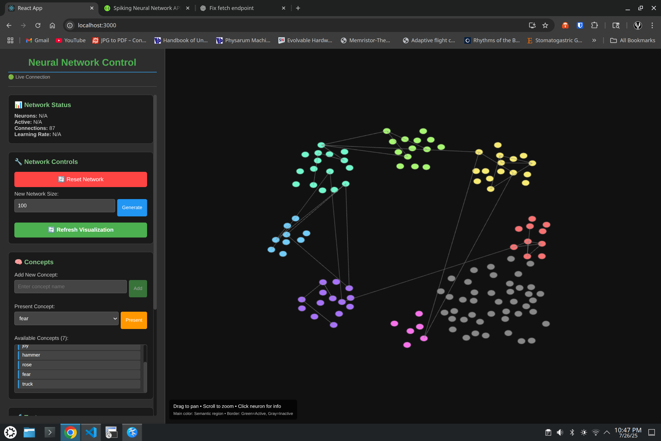
The validation pipeline is the part I’m proudest of. The same network architecture is exercised at multiple scales — 300 neurons (the earlier paper), 7,500 neurons (the ASSOCIATIVE region in isolation), and 25,100 neurons (the full hierarchical architecture) — and behavior is compared across scales to confirm that nothing fundamental changes as the network grows. The architecture is meant to scale; the framework’s job is to prove that it does.

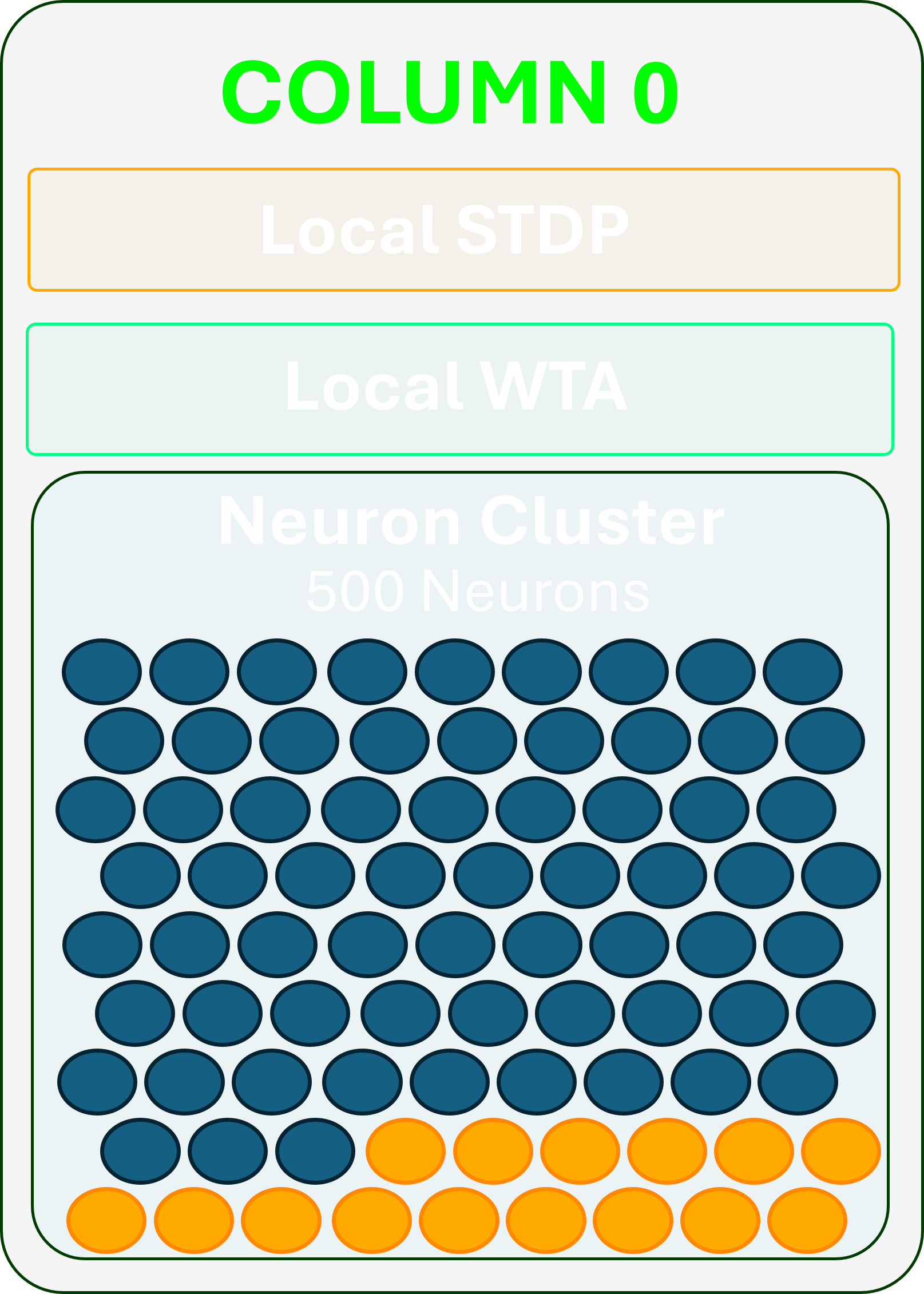
What “behavior comparison across scales” means in practice. Three metrics carry across all scales: pattern distinctiveness (mean pairwise overlap between stored concepts), mean instantaneous sparsity (the fraction of neurons firing per 1 ms timestep, which sets average power), and cued recall accuracy. The 300-neuron version achieved 65–67% distinctiveness with 0.39% instantaneous sparsity and 100% completion from 30% cues across 50 patterns; the 25,100-neuron version achieves 83.1% distinctiveness at 0.71% instantaneous sparsity with 80% cued recall across 993 concepts. The scaling is non-trivial — the smaller network’s columnar encoding (3 columns × 100 neurons) is replaced by 15 columns × 500 neurons in the ASSOCIATIVE region — but the qualitative behavior (distributed columnar attractor formation, gradual capacity degradation rather than catastrophic interference, sparse instantaneous activity) holds across both. Where the small network exhibited something the large one didn’t (or vice versa), we treated it as a bug to chase, not a result to publish.

This kind of cross-scale validation isn’t standard in the field. Most analog SNN papers report results at a single scale and call it a day. Doing it at multiple scales pays off in two ways: it catches implementation bugs that only show up under load (one example: a synapse accumulator overflow that didn’t fire below ~3,000 neurons), and it builds defensible confidence that the architecture will scale to silicon densities — millions of neurons per die — without surprises.

Encoding: from text to spikes via hyperbolic geometry

A spiking neural network can’t read English. To get something useful into the substrate, you need to turn it into spikes — and the encoding choice matters a lot. The pipeline NeuroMatrix uses for text goes through hyperbolic geometry, which is a less common choice than it should be.

The pipeline:

text → sentence-transformer (384D Euclidean)
     → hyperbolic Poincaré ball embedding (8D)
     → spike pattern generation
     → C++ SNN substrate

Step 1: text → 384D Euclidean. A standard sentence-transformer model (the kind that produces embeddings for semantic search) turns a word or phrase into a 384-dimensional vector. Standard ML, off-the-shelf, well-understood.

Step 2: 384D Euclidean → 8D Poincaré. The 384D vector is projected into an 8-dimensional Poincaré ball — the standard model of hyperbolic space, where the entire infinite hyperbolic plane is mapped into a finite ball with distances that grow exponentially as you approach the boundary. The point of the projection isn’t dimensionality reduction; it’s that hyperbolic space encodes hierarchy naturally. In Euclidean space, the number of points at distance r from any other point grows polynomially. In hyperbolic space, it grows exponentially — exactly matching how a tree branches as you go down its levels. Concepts that are hierarchically related (dog is a kind of mammal is a kind of animal) end up at corresponding depths in the ball; semantically related concepts cluster locally; the geometry does work that Euclidean embeddings have to learn the hard way.

Step 3: 8D Poincaré → spike pattern. Each of the 8 coordinates maps to a population of input neurons in the ASSOCIATIVE region’s input layer (1,200 input neurons total). Coordinate values are converted to firing rates over a 100 ms encoding window; concepts with similar hyperbolic embeddings produce similar spike patterns, and the network’s STDP learning forms attractor basins around those patterns.

Vector database. The 8D Poincaré embeddings for all 993 concepts are stored in a hyperbolic vector database so they can be queried by similarity (geodesic distance in the ball) rather than just retrieved by ID. This is what closes the loop from “user asks a question in English” to “network recalls the closest learned concept” without going through an LLM at the retrieval step. The LLM only re-enters at the output stage, if natural language is what the user wants back.

The encoding pipeline is implemented for text in the current system. Audio and visual paths are architecturally defined (rod/cone → edge detection → object → scene parallels the cortex’s V1 → V2 → V4 → IT hierarchy) but not yet built; that’s downstream work.

Results: associative memory at scale

To validate the architecture against a meaningful task, we implemented sparse associative memory — a network that learns concepts and recalls them from partial cues. It’s the simplest cognitive task you can give a network and it’s the one Hopfield originally used to characterize the capacity of recurrent networks back in 1982.

The headline numbers from the paper:

• 993 concepts stored in the 25,100-neuron architecture (specifically in the ASSOCIATIVE region: 7,500 neurons across 15 cortical columns, with 1,200 input neurons)
• 83.1% ± 3.7% distinctiveness across all 993 concepts, reaching 96% of the Hopfield capacity limit — the theoretical maximum number of patterns a network of this size can store before retrieval breaks down
• 80% cued recall accuracy on the full 993-concept set; 100% cued recall at 200 concepts
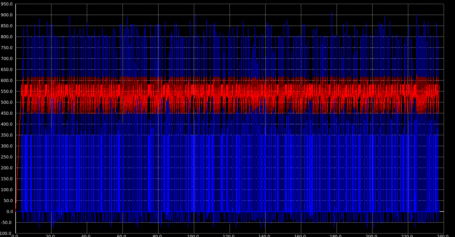
• 0.71% mean instantaneous sparsity — typically fewer than 200 of the 25,100 neurons firing per millisecond, keeping per-timestep power consistent with analog neuromorphic operation
• Energy per spike: 7.2 pJ under PSP 103.6 (dominated by ½·Cmem·VDD²)

Interpretation. The 96%-of-Hopfield number deserves context. Classical Hopfield networks collapse catastrophically beyond their capacity limit — store one pattern too many and retrieval breaks down across all stored patterns. NeuroMatrix’s distributed columnar encoding (15 cortical columns, sparse 0.3–1.0% feedforward connectivity) avoids this: distinctiveness stabilizes above 83% from 300 concepts onward and shows no monotonic decline through 993, achieving a storage ratio of 0.132 (993 / 7,500) that approaches the classical 0.138 N reference bound despite an entirely different architecture — spiking LIF neurons instead of binary units, multiplicative STDP instead of Hebbian learning, sparse columnar connectivity instead of full connectivity. The result isn’t that we beat Hopfield’s bound (we don’t — it’s a reference, not a hard limit for our architecture). It’s that a hardware-realistic analog network with all the constraints that implies — finite weight precision, device mismatch, subthreshold leak currents — gets close to a bound usually quoted only for idealized recurrent networks.

The 20% gap to perfect cued recall at full scale is real and worth being honest about. The 100 ms observation window matters (recall drops to 47% at 30 ms), the cue-informed paradigm assumes you know which concept you’re cueing (uncued free recall would be much harder), and individual concept similarity in the embedding space puts a floor on how distinct stored patterns can be. None of those is a defect in the network so much as a property of the task; a real cognitive system would integrate multiple cues and contextual priors before committing to a recall, and the framework supports that. But the 80% number is the bare 5-sample, 10 ms cued recall against 993 concepts in isolation, and that’s what we report.

The cognitive stack

The 25,100-neuron architecture in the paper is built around five regions — ASSOCIATIVE, SEQUENTIAL, LOGIC, CAUSAL, PLANNING — that together form NeuroCog, the cognition module. ASSOCIATIVE is the one validated in the MWSCAS paper; the other four are architecturally defined (region topology, WTA parameters, STDP rates set) but not yet validated at scale. That’s the immediate next step.

NeuroCog isn’t the only module sitting on the NeuroMatrix substrate. The longer plan is a stack of cognitive modules, each with its own internal hierarchy, all running on the same Axon-Hillock LIF substrate and communicating via AER (Address-Event Representation — the standard event-routing protocol for neuromorphic systems).

NeuroCog — general cognition, currently the most-developed module:

• Associative — pattern memory; the validated region (993 concepts, 96% Hopfield)
• Sequential — temporal sequence learning, ordering and prediction
• Logic — combinatorial reasoning over learned concepts
• Causal — cause/effect relationships, intervention modeling
• Planning — goal-directed search over the learned concept graph

Linguistic — language understanding, mirroring the levels at which humans process language:

• Phonetics — sound-to-token mapping
• Morphology — word-internal structure
• Syntax — grammatical relations
• Semantics — meaning, where this module hands off to NeuroCog’s associative layer
• Pragmatics — context and intent

Generative — production, the inverse direction of Linguistic:

• Lexical — word selection
• Syntactic — sentence-level construction
• Narrative — multi-sentence coherence

Episodic — memory of specific events, distinguished from NeuroCog’s associative semantic memory by being temporally indexed; encodes, stores, and consolidates event traces with their temporal context, mirroring how hippocampal-cortical interaction works in biology.

Each module has the same internal structure pattern: hierarchical regions, WTA competition within columns, STDP learning, sparse columnar connectivity, AER routing between regions and between modules. The modules are stamped from the same architectural template; what differs is the connectivity, the region sizes, and the input/output bindings.

The end-to-end stack — text input → encoding pipeline → Linguistic → NeuroCog (associative + sequential + logic) → Generative → text output, with Episodic running alongside and consolidating events — has been demonstrated on the existing tech stack with a generated sentence and persistent memory of the inputs that produced it. That demonstration is preliminary and not yet published; the MWSCAS paper covers the substrate and the associative region only, which is the foundation everything else depends on.

What’s next

Several threads pull forward from here, with different timelines and different levels of how-real-this-is.

Validating the other NeuroCog regions. SEQUENTIAL, LOGIC, CAUSAL, PLANNING are architecturally defined. The next concrete milestone is validating each at scale with metrics analogous to what we have for ASSOCIATIVE (capacity, distinctiveness, recall fidelity). This is in-progress work using the same simulation infrastructure.

The Fabrica toolchain. Building NeuroMatrix exposed how brittle existing analog EDA workflows are for networks of this size. Most analog tools assume you’re laying out one block at a time, by hand; we need to lay out tens of thousands of neurons and millions of synapses with consistent characterization across them. Fabrica is the toolchain we’re building to make that possible — the Circuit IR, the EKV/PSP verification bindings, the visualization layer (Fabrica-Viz) that generates the schematic figures in the paper. Fabrica gets its own writeup.

Tape-out. Aspirational at the moment. The circuit is validated in simulation across three fidelity levels including foundry-accurate PSP 103.6, but the immediate focus is making Fabrica and the framework production-ready and validating the remaining cognitive modules. A real tape-out via IHP’s shuttle service is downstream of that — months to years out, not weeks. I’d rather say so honestly than gesture at a timeline I can’t commit to.

The bigger picture: a cognitive coprocessor. The long-term goal isn’t to replace a GPU; it’s to sit next to one. Imagine a PCIe accelerator card with a million analog neurons doing event-driven sparse computation alongside a conventional CPU/GPU that handles dense workloads. The card’s bandwidth requirement is low because only the spikes cross the PCIe boundary — and spikes are sparse by construction (0.71% activity means a 1M-neuron card produces ~7,000 events per millisecond, well within PCIe’s reach). The host sees an associative knowledge store with continuous learning built in, accessed via a thin API. Pair it with an LLM that handles natural language at the I/O boundary and you have a system that learns from every interaction without retraining, that holds episodic memory of specific conversations, and that grounds its language understanding in a continuously-updated semantic network. That’s the vision. NeuroMatrix is the first checkpoint.

Co-authors and credits

This is a team project, and the team is small enough to name everyone.

• Noah Sabra — paper co-author; LIF neuron design, circuit build, and verification work. The Axon-Hillock topology choice and its PSP 103.6 validation went through Noah’s hands as much as mine.
• Michael Baker — paper co-author; synapse design — the STDP implementation, weight dependence dynamics, and the sparse columnar connectivity scheme that lets the network avoid catastrophic interference.
• Dr. Claudio Talarico — faculty advisor, analog VLSI.
• Prof. Graham Morehead — faculty advisor.

Funding and infrastructure support from Gonzaga University. The simulation pipeline runs on the NCS cluster, which is my own infrastructure — 12 nodes, 96–128 GB DDR3 each, k3s-orchestrated, built specifically to handle the 25,100-neuron simulations the laptop couldn’t.

The paper is currently under review at MWSCAS 2026. I’ll link the final PDF here once it’s published; in the meantime, the preprint is available on request — email me.