Fabrica

Why this exists

Existing analog EDA tools — Cadence Spectre, Synopsys HSPICE, ngspice, Xyce — are excellent at what they were designed for: simulating a few hundred to a few thousand devices with maximum fidelity. They’re not designed for what neuromorphic computing needs, which is a network of tens of thousands of small, near-identical analog blocks that need to be designed, validated, and laid out as a system rather than as individual circuits.

Two specific frictions kept showing up while I was working on NeuroMatrix. First, the iteration loop was wrong. If I wanted to test a new neuron topology in a network, I had to lay out the schematic in Virtuoso, set up the simulation manually, wait for it to run, post-process the results in Python, and then loop back to the schematic. Even a small change took fifteen minutes. For a network architect making hundreds of small design decisions, that’s unworkable.

Second, the validation story was incoherent. Behavioral models (Verilog-A, Python prototypes) and SPICE-level transistor models don’t share a representation. You write the network architecture twice — once in your prototype, once in your SPICE netlist — and there’s no automated way to confirm they’re describing the same circuit. Bugs hide in the gap.

The third friction is the one that actually pushed me to build my own tool. I wanted a single workflow that could do all three things at once: run behavioral tests on a network architecture to analyze capacity and associative dynamics at scale (which demands the simulator be fast), use a general analog model — EKV or similar — to validate the circuit physics without locking to a foundry yet (which needs SPICE-like fidelity at iteration speed), and then drop into foundry-accurate modules like IHP’s PSP 103.6 when I needed to commit. Each tier exists separately in the ecosystem; nothing strings them together against the same circuit description. I tried building that workflow on top of existing tools for a while. The amount of glue code I was writing made it clear that the glue was the actual problem, and I might as well build the thing the glue was reaching for.

Fabrica is the answer to those frictions: one circuit description, three execution tiers, fast iteration at the top tier, foundry fidelity at the bottom, automatic consistency checks across all of them.

The three tiers

The architecture is built around three execution backends that compile from a single intermediate representation:

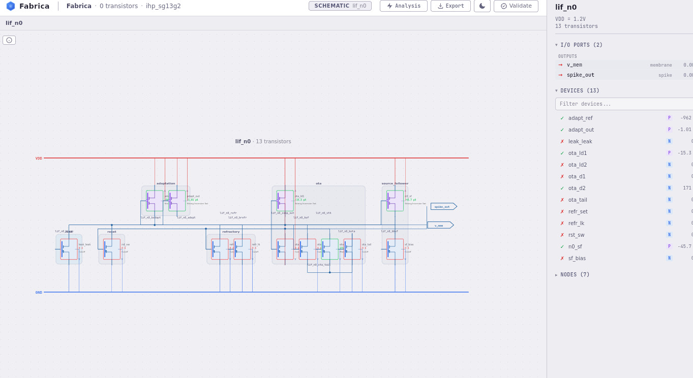
Tier 1: behavioral

Pure Python, no physics. A neuron is described by its differential equations:

class LIFNeuron(Behavioral):
    def equations(self):
        return [
            dV_dt == (I_in - V / R_leak) / C_mem,
            spike == (V > V_threshold),
        ]

The behavioral tier exists to let you reason about the architecture, not the implementation. Does this network learn? Does it converge? Does the population code make sense? Run it on your laptop in a Jupyter notebook, sweep parameters in seconds, iterate on the algorithm. No transistors, no foundry models, no SPICE netlist.

This is the tier where 95% of the iteration happens. The other two tiers are validation gates, not design surfaces.

Tier 2: generic analog (EKV 2.6)

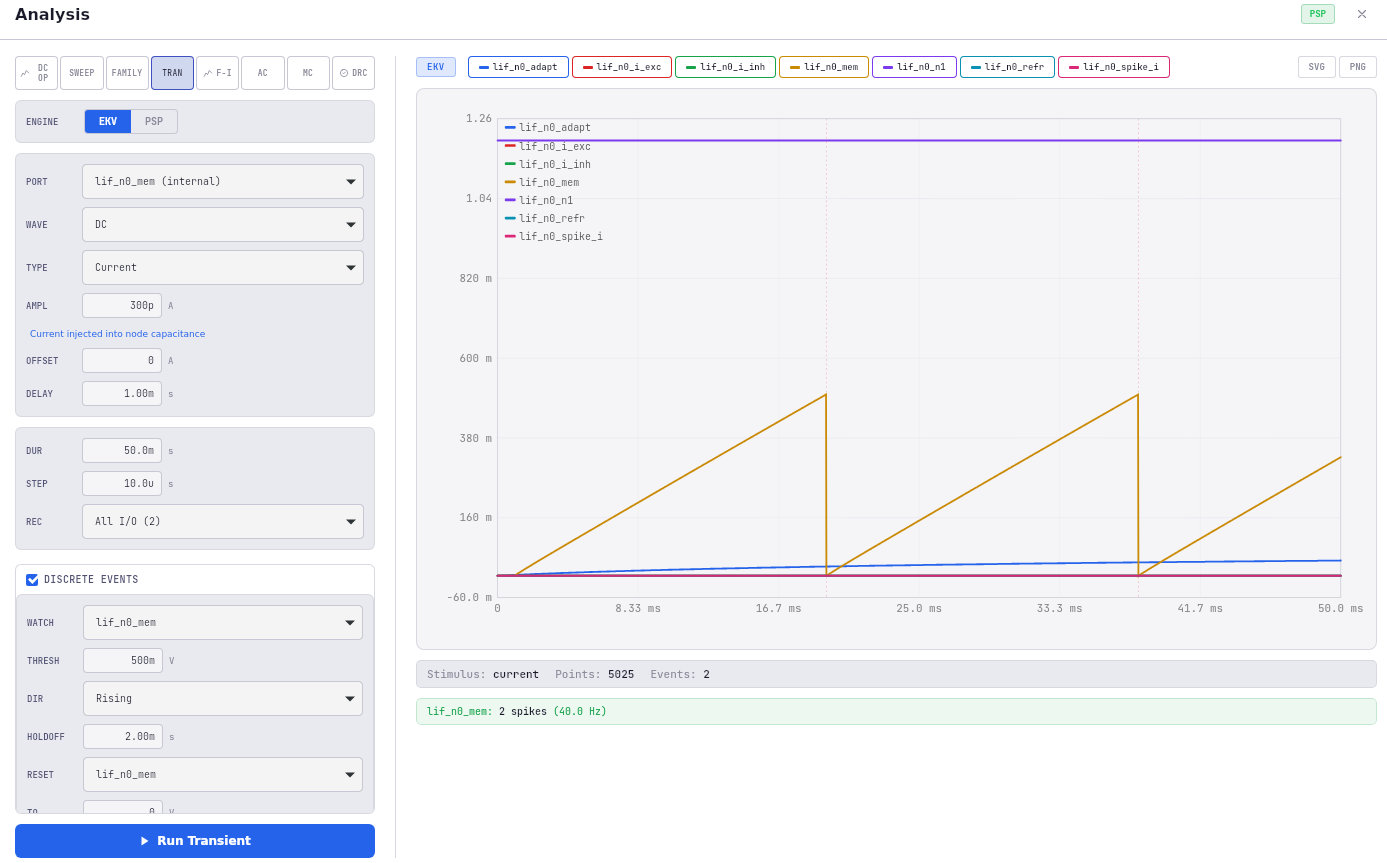
The generic-analog tier introduces real circuit physics, but using process-independent device models. Transistors are EKV 2.6 — a compact MOSFET model designed for analog simulation that’s parameterized by a handful of physical quantities (threshold, transconductance, channel length modulation) rather than a thousand-line PDK card.

Why EKV over BSIM. BSIM is the foundry-standard family of MOSFET models — what almost every commercial PDK ships. It’s also a nightmare to reason about: hundreds of parameters, branching equations stitched together across operating regions, and most importantly, discontinuities at the boundaries between regions. The BSIM equations for weak inversion (subthreshold) are a different analytical formulation from strong inversion, and they’re patched together at the boundary with smoothing functions that aren’t truly continuous in higher derivatives. For digital circuits that swing rail-to-rail through saturation, none of this matters — you’re never sitting on the boundary. For analog neuromorphic circuits that live in subthreshold and only briefly pass through the boundary during a spike, the discontinuity is a numerical landmine. The solver wastes timesteps converging across it; the analytic Jacobian becomes a piecewise object instead of a smooth one; small parameter changes produce simulation artifacts that don’t correspond to real circuit behavior.

EKV is a single set of equations valid from deep subthreshold all the way through strong inversion. The model is C∞ continuous through the operating regions — derivatives of every order exist and are smooth. For a neuromorphic LIF circuit where the membrane voltage spends most of its time in subthreshold and the interesting dynamics happen exactly at the boundary, that’s not a nice-to-have; it’s load-bearing. Choosing BSIM would have meant either accepting numerical artifacts or writing extensive smoothing on top, which defeats the purpose of using a foundry-standard model in the first place.

The generic-analog tier answers a different question than the behavioral tier: does this circuit work as an analog circuit, independent of process? If your LIF neuron only spikes correctly when you assume threshold voltages match to 0.1%, you can’t fabricate that. The generic-analog tier catches those problems before you’ve committed to a PDK.

Tier 3: foundry-accurate (IHP PSP 103.6)

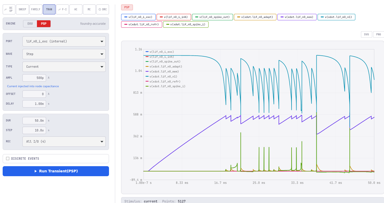
The bottom tier uses PSP 103.6 models from IHP’s SG13G2 130nm BiCMOS process. PSP is the surface-potential-based MOSFET model used in modern foundry PDKs; it captures the full set of process effects — gate leakage, junction capacitance, mismatch, temperature, the long tail of second-order effects that matter at silicon.

At this tier, you’re doing what a conventional SPICE simulator does, with one important difference: the network description is exactly the one you simulated in tiers 1 and 2. You haven’t rewritten anything. You’re not validating a netlist transcription; you’re validating that the same architecture, under foundry-accurate physics, still does what your prototype said it would.

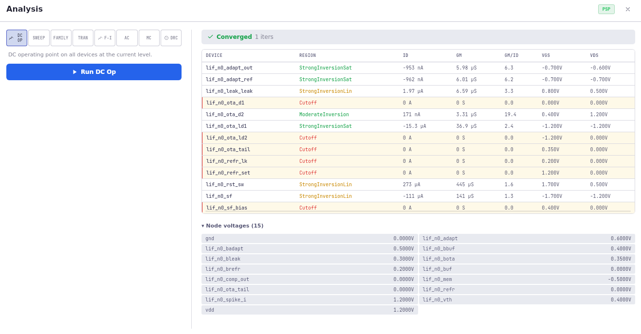
The canonical “tier-3 caught it” story comes from NeuroMatrix. An earlier version of the LIF neuron used an OTA-based comparator topology — an operational transconductance amplifier sensing the membrane voltage and tripping a digital output. EKV 2.6 simulations of that topology looked correct: clean spikes, plausible firing rates, well-behaved across bias sweeps. PSP 103.6 told a different story. Under the foundry-accurate model — which captures gate-induced drain leakage (GIDL) and junction leakage that EKV 2.6 idealizes away — the OTA had a stable DC equilibrium that pinned the membrane voltage just below threshold. The neuron wouldn’t spike at all, even under what should have been suprathreshold stimulus, because real-silicon leakage was holding it in place. EKV had no way to see this; PSP did. We revised the topology to the Axon-Hillock design that’s now in the paper. Without tier 3, that bug would have been a tape-out failure.

The three tiers also have wildly different runtimes. The behavioral tier is built for speed and runs interactively; the EKV tier is comparable to a fast SPICE simulator; the PSP tier is the slowest and most expensive — overnight runs are normal for full-network sweeps. The tradeoff is intentional: you only pay foundry-accurate cost when you’ve earned the right to, by passing the cheaper tiers first.

The IR — one description, three backends

The whole three-tier approach only works because of a deliberate intermediate representation. Every circuit in Fabrica is first lowered to a Circuit IR — a typed graph of devices, nodes, and parameters with a stable schema and explicit versioning.

The IR has a few properties worth naming:

• Hierarchical. You describe a neuron once; the network reuses it 25,000 times without re-elaborating.
• Versioned. The schema migrates forward with explicit migration rules, so case studies written against an older Fabrica still load.
• Backend-agnostic. The IR itself knows nothing about EKV, PSP, or behavioral models. Each backend has its own lowering pass that consumes the IR and produces what it needs.
• Inspectable. You can dump the IR to disk as JSON or a structured text format and diff two versions of a circuit by hand.

This is unglamorous infrastructure work and most of Fabrica’s value lives here. The user-facing Python API is thin; the IR is what makes the three-tier story coherent.

Hierarchical netlisting matters. At 25,000 neurons with 525,000 synapses, a flat netlist either runs out of memory during elaboration or wastes hours re-emitting the same neuron netlist twenty-five thousand times. Conventional SPICE simulators handle hierarchy through subcircuit calls (.subckt), but the references are textual and the simulator still has to flatten the hierarchy internally before solving. Fabrica’s IR keeps the hierarchy as a first-class structure all the way through to the solver: one neuron definition exists in memory; 25,000 references point at it; the sparse Jacobian is built block-wise rather than reconstructed from scratch each timestep. Memory footprint scales with the number of unique subcircuits, not the number of instances. For neuromorphic networks where the same neuron is repeated tens of thousands of times, that’s the difference between “fits on the cluster” and “doesn’t fit anywhere.”

The numerical core

The interesting engineering — and most of the test surface — is in the EKV-tier solver. The constraint: the same kernel needs to handle 100 transistors and 25,000 transistors with the same numerical correctness.

The shape of the solver:

• Sparse representation — at 25k devices the Jacobian is ~99.9% zeros; treating it as dense is a non-starter
• ILU-preconditioned BiCGSTAB — iterative sparse linear solver that converges on the kinds of ill-conditioned matrices analog circuits produce. ILU (incomplete LU) is the preconditioner that makes BiCGSTAB converge in tens of iterations instead of thousands
• Analytic Jacobian — EKV’s equations are differentiable in closed form, so we compute exact partial derivatives instead of approximating via finite differences. Faster and more numerically stable
• LTE-controlled timestep — local truncation error estimation lets the simulator take large steps through quiet regions of the simulation (between spikes) and small steps through fast transitions (during a spike). The naïve fixed-timestep approach either runs forever or misses spike detail

The integration story. Early versions of the transient engine used the trapezoidal rule, the textbook implicit second-order method that every SPICE simulator ships. Trapezoidal is correct, conservative, and energy-preserving in a way that matters for oscillatory circuits — none of which is what a LIF network needs. LIF dynamics are dissipative (charge leaks off the membrane), the system is stiff (the spike happens on a microsecond timescale while integration happens on a millisecond timescale), and the trapezoidal rule is famously prone to trapezoidal ringing: spurious oscillations at half the sampling frequency when the integrator hits a discontinuity. Every spike in a LIF network is a discontinuity. The trapezoidal engine wasn’t slow because the math was slow; it was slow because it was constantly retrying timesteps that had developed numerical oscillations the LTE controller correctly flagged as bad.

Backward Differentiation Formulas (BDF) don’t have this problem. BDF-1 is implicit Euler; BDF-2 is a second-order method that’s L-stable — it actively damps oscillations rather than preserving them — and it handles stiff systems gracefully. Switching the transient engine from trapezoidal to BDF-1/BDF-2 (the engine picks dynamically based on the local stiffness) cut the 50 ms LIF simulation from ~37 seconds to 0.135 seconds, the ~274× speedup. The engine wasn’t faster per timestep; it was retrying far less.

The 274× speedup over the previous trapezoidal implementation is the kind of number that looks like a typo. It isn’t. The trapezoidal-rule version was correct but spent most of its compute time on a stability problem that BDF-2 doesn’t have — the engine wasn’t slow, it was retrying. The lesson is that algorithmic choices matter more than micro-optimization for this kind of work.

Why C++, Rust, and Python

Three languages for one framework is unusual, and worth justifying.

C++ is the numerical core. The EKV solver, the IR data structures, the sparse linear algebra. Everything performance-critical lives here. C++ wins on Eigen integration, decades of battle-tested numerics libraries, and predictable memory layout for sparse matrices.

Rust hosts the Circuit IR and the Fabrica EDA bindings — the same role it plays in the broader NeuroMatrix stack. The IR is the contract between the front-end (Python, where users write networks) and the back-end (C++, where networks get solved), and Rust is the right language for that contract: memory-safe by construction so the IR can’t be corrupted by aliasing bugs, ergonomic enum/struct types that match the IR’s algebraic-data-type shape, and good interop in both directions. The IR’s stability across schema versions, hierarchical references, and backend-agnostic lowering passes are all easier to enforce in Rust’s type system than in either C++ or Python.

Python is the user surface. Anything a circuit designer writes is in Python — network descriptions, parameter sweeps, results analysis. nanobind binds the C++ core (faster and lighter than pybind11 for this use case). The CLI lives at this layer too, though it’s still being wired up.

The split isn’t accidental. Each language does what it’s best at: C++ for inner loops, Rust for the IR and the type-level guarantees that come with it, Python for the language a researcher actually wants to write in. The connection points — nanobind for Python↔C++, and cbindgen for Rust↔C++ (Rust generates a C header; C++ links against it through extern "C") — are explicit and minimal. Anything crossing a language boundary crosses a deliberate API surface, not a leaky one.

The C ABI

One detail that often gets skipped in toolchain writeups: there’s a C ABI layer under all of this. fabrica_v1.h exposes ten functions with stable signatures for opening a circuit, lowering it through the IR, configuring a backend, running a simulation, and reading results.

Why a C ABI matters: it’s the universal contract. The Python bindings are written against it. The Rust orchestration is written against it. If someone wants to embed Fabrica in a different host language — Julia, MATLAB, a notebook environment — they only need to bind ten functions. The C++ implementation is free to refactor as long as the ABI stays stable.

Versioning. The v1 in the filename is doing work. The plan is per-symbol versioning: each exported function carries its ABI version (fabrica_open_circuit_v1, fabrica_run_transient_v1, etc.), with new versions added side-by-side rather than replacing old ones. A future v2 ABI lives in fabrica_v2.h as new symbols; v1 callers keep working until they’re explicitly migrated. This is the GNU libc approach and the one battle-tested across decades of binary compatibility — heavy for a research tool, but the cost of getting it wrong is rebuilding every downstream caller every time the internals change, and that’s the cost I’m trying to avoid.

Testing

345+ tests across C++, Python, and Rust, last I counted. The test surface breaks down roughly:

• C++ unit tests for the IR, the lowering passes, the solver kernels, and the integration routines. Heavy use of property-based testing for the numerics — given a circuit that obeys conservation of charge, the simulator’s output must obey it too, modulo numerical tolerance.
• Cross-tier consistency tests — the most important set. The same behavioral circuit, the same EKV circuit, and the same PSP circuit are simulated, and their outputs are compared at agreed-upon interfaces (spike times, mean firing rate, equilibrium voltages). If they diverge beyond tolerance, something is wrong somewhere.
• Python integration tests that exercise the full path from network description to results.
• Rust tests for the IR itself — schema migration round-trips, hierarchical reference resolution, cbindgen header generation, lowering-pass correctness against known-good output. The Rust suite is where the type-level guarantees actually get exercised; if a property holds in the Rust types, the tests assert it holds at runtime too.

The cross-tier consistency tests are the load-bearing infrastructure. Without them, the three-tier story is unfalsifiable — you can’t claim “the same architecture works across all three tiers” if you’ve never automated checking it.

What’s done, what’s next

The roadmap, as honestly as I can put it:

Done:

• IR schema, migrations, hierarchical netlisting
• EKV 2.6 sparse solver with ILU+BiCGSTAB, analytic Jacobian, LTE timestep
• BDF-1/BDF-2 transient integration replacing the old trapezoidal engine
• Multi-block analysis (DC operating point, AC small-signal, transient)
• C ABI v1, ten core functions
• 345+ tests across three languages

In progress:

• Section 5: EKV/PSP multi-engine consistency tests — the cross-tier validation work that proves the three-tier story actually holds
• Section 10: error handling audit, replacing ad-hoc error returns with a consistent error model across the C ABI
• Python nanobind bindings update to track the v1 ABI
• CLI wiring (the framework currently runs from Python scripts; the CLI is meant to be the front door for non-Python workflows)
• Fabrica-Viz updates (the companion visualization tool that generates the schematic figures in the NeuroMatrix paper)

Open problems:

• DAE split for stiff mixed fast/slow node topology. A network of LIF neurons has fast dynamics (the spike itself, microseconds) coexisting with slow dynamics (subthreshold integration, milliseconds). Treating the whole system with a single timestep wastes compute on the slow nodes and under-resolves the fast ones. The right approach is a differential-algebraic equation split: integrate fast nodes with a small step, slow nodes with a large step, coordinate at the interfaces. Easy to describe; hard to implement without introducing artifacts at the interface (timestep mismatches show up as energy conservation errors that look exactly like bugs). The literature on multirate integrators is dense and most of it assumes a clean partition between fast and slow that LIF networks don’t actually have — adaptation currents move between fast and slow as the network state evolves. I’ve sketched a few approaches; none have survived the cross-tier consistency tests yet. Working on it.

What this is, what it isn’t

Fabrica isn’t going to compete with Spectre on general analog circuit simulation. It isn’t trying to. It’s a tool for one specific class of problem — large, hierarchical, near-uniform analog networks — built by someone who needed that tool and couldn’t find it.

Whether it ends up useful to anyone else is an open question. The architecture is general enough that it should: any analog system with a lot of repeated structure and a need to validate across abstraction levels should fit. But I built it for myself, and proving generality means finding someone else’s project that fits, and that hasn’t happened yet.

For now, it’s the toolchain behind NeuroMatrix, and that’s enough.

If you’re working on similar problems and want to talk about toolchain architecture, the cross-tier consistency strategy, or the BDF/DAE-split work — email me. I’d rather compare notes than maintain a tool alone.